- https://users.cs.duke.edu/~cynthia/
- http://wilkeraziz.github.io/pages/landscape
- https://probcomp.github.io/Gen/
- https://m-clark.github.io/workshops.html
- https://dsteinberg.github.io/pages/research-projects.html
- https://tminka.github.io/papers/index.html
- http://am207.info/resources.html
- http://mlg.eng.cam.ac.uk/tutorials/07/
- http://pandamatak.com/people/anand/771/html/html.html
- https://www.cs.princeton.edu/courses/archive/fall11/cos597C/
- O'Bayes 2019: Objective Bayes Methodology Conference
- Bayesian Learning for Machine Learning: Part I
- Philosophy of Bayesian Inference, Radford M. Neal, January 1998
- Understanding computational Bayesian statistics
- Variational Methods for Bayesian Independent Component Analysis by Rizwan A. Choudrey
- PROBABILISTIC-NUMERICS.ORG
- Variational Bayes for Implicit Probabilistic Models
Bayesian learning can be regarded as the extension of Bayesian statistics. The core topic of Bayesian learning is thought as prior information to explain the uncertainty of parameters.
It is related with Bayesian statistics, computational statistics, probabilistic programming and machine learning.
- [Bayesian] “我是bayesian我怕谁”系列 - Gaussian Process
- Bayesian Learning
- Lecture 9: Bayesian Learning
- Bayesian Learning
- Bayesian machine learning
- Infinite Mixture Models with Nonparametric Bayes and the Dirichlet Process
- Bayesian Learning for Machine Learning: Part I - Introduction to Bayesian Learning
- Bayesian Learning for Machine Learning: Part II - Linear Regression
- Bayesian Learning by Burr H. Settles, CS-540, UW-Madison, www.cs.wisc.edu/~cs540-1
- Bayesian machine learning @fastML
- Understanding emprical Bayesian hierarchical learning
- While My MCMC Gently Samples - Bayesian modeling, Data Science, and Python
- Probabilistic Models in the Study of Language
- Statistical Rethinking A Bayesian Course with Examples in R and Stan (& PyMC3 & brms too)
- COS597C: Advanced Methods in Probabilistic Modeling
- COS513: Foundations of Probabilistic Modeling
- CSSS 564: Bayesian Statistics for the Social Sciences (University of Washington, Spring 2018)
- Radford Neal's Research: Bayesian Inference
- Learn Bayesian statistics
- http://ryanrossi.com/search.php
- https://bayesianwatch.wordpress.com/
| Bayes Formulae | Inverse Bayes Formulae |
|---|---|
Naive Bayes is to reconstruct the joint distribution of features and labels naive idea is to simplify the computation process by assumption that the features are conditional independence so that
$$
Pr(\vec{X}\mid y) =\prod_{i=1}^{p} Pr(\vec{X}^{(i)}\mid y).\tag{1}
$$
And the predicted labels will be computed via $$ Pr(y\mid \vec{X}) = \frac{Pr(y) Pr(\vec{x}\mid y)}{\sum Pr(y)Pr(\vec{x}\mid y)}. \tag{2} $$
where the conditional probability
The prior probability
- Not so naive Bayes: Aggregating one-dependence estimators
- https://link.springer.com/article/10.1007%2Fs10994-005-4258-6
Approximate Rejection Algorithm:
- Draw
$\theta$ from$\pi(\theta)$ ;- Simulate
$D′ \sim P(\cdot\mid \theta)$ ;- Accept
$\theta$ if$\rho(D, D')\leq \epsilon$ .
- Symposium on Advances in Approximate Bayesian Inference, December 2, 2018
- RIKEN Center for Advanced Intelligence Project: Approximate Bayesian Inference Team
- Approximation Methods for Inference, Learning and Decision-Making
- Algorithms and Theoretical Foundations for Approximate Bayesian Inference in Machine Learning
- APPROXIMATE BAYESIAN INFERENCE
- Approximate Bayesian Computation: a simulation based approach to inferenc
- Approximate Bayesian Inference for Latent Gaussian Models Using Integrated Nested Laplace Approximations
- Approximate Bayesian inference via synthetic likelihood for a process-based forest model
- A family of algorithms for approximate Bayesian inference by Thomas Minka, MIT PhD thesis, 2001
- EnLLVM – Fast Approximate Bayesian Inference
- approximate Bayesian inference under informative sampling
- Approximate Bayesian Inference Reveals Evidence for a Recent, Severe Bottleneck in a Netherlands Population of Drosophila melanogaster
- Approximate Bayesian inference methods for stochastic state space models
- A roadmap to research on EP
- https://en.wikipedia.org/wiki/Expectation_propagation
- http://www.mbmlbook.com/TrueSkill_A_solution__expectation_propagation.html
- Variational-Bayes .org
- A tutorial on variational Bayesian inference
- The Variational Bayesian EM Algorithm for Incomplete Data: with Application to Scoring Graphical Model Structures
- Variational Inference: A Review for Statisticians
- Another Walkthrough of Variational Bayes
- The Variational Approximation for Bayesian Inference
- High-Level Explanation of Variational Inference by Jason Eisner (2011)
- VBA (Variational Bayesian Analysis): Interpreting experimental data through computational models
We consider a multilevel model to be a regression (a linear or generalized linear model) in which the parameters—the regression coefficients—are given a probability model. This second-level model has parameters of its own—the hyperparameters of the model—which are also estimated from data. The two key parts of a multilevel model are varying coefficients, and a model for those varying coefficients (which can itself include group-level predictors). Classical regression can sometimes accommodate varying coefficients by using indicator variables. The feature that distinguishes multilevel models from classical regression is in the modeling of the variation between groups.
Multilevel models are also called hierarchical, for two different reasons: first, from the structure of the data (for example, students clustered within schools); and second, from the model itself, which has its own hierarchy, with the parameters of the within-school regressions at the bottom, controlled by the hyperparameters of the upper-level model.
Hierarchical Bayes:
- explicitly represent category hierarchies for sharing abstract knowledge.
- explicitly idenAfy only a small number of parameters that are relevant to the new concept being learned.
Hierarchical Bayesian Regressionextends the Bayesian models by setting the uncertainty of the uncertainty such as $$ y\sim Pr(\phi(x)\mid \theta)\ Pr(\phi(x)\mid \theta) = \frac{Pr(\theta\mid\phi(x))Pr(\phi(x))}{P(\theta)}\ Pr(\phi(x))= Pr(\phi(x)\mid \eta) Pr(\eta)\ \vdots $$
We can take any factor into consideration in this hierarchical Bayesian model. And it is a graphical probability model, which consists of the connections and probability.
- https://twiecki.io/
- The Best Of Both Worlds: Hierarchical Linear Regression in PyMC3
- Hierarchical Bayesian Neural Networks with Informative Priors
- https://www.cnblogs.com/huangxiao2015/p/5667941.html
- https://www.cnblogs.com/huangxiao2015/p/5668140.html
- BAYESIAN HIERARCHICAL MODELS
- Chapter 4: Regression and Hierarchical Models
- GLM: Hierarchical Linear Regression
- Understanding empirical Bayesian hierarchical modeling (using baseball statistics) Previously in this series:
- Probabilistic Model in the Study of Language
- https://www.wikiwand.com/en/Bayesian_hierarchical_modeling
- SAS/STAT Examples Bayesian Hierarchical Poisson Regression Model for Overdispersed Count Data
- Hierarchical Regression and Spatial models
- Short Course for ENAR 2009 - Sunday, March 15, 2009: Hierarchical Modeling and Analysis of Spatial-Temporal Data: Emphasis in Forestry, Ecology, and Environmental Sciences
- Doing Bayesian Data Analysis
- Bayesian methods for combining multiple Individual and Aggregate data Sources in observational studies.
- https://www.stat.berkeley.edu/~census/goldbug.pdf
- http://www.biostat.umn.edu/~ph7440/pubh7440/Lecture5.pdf
- CS&SS/STAT 564: Bayesian Statistics for the Social Sciences, University of Washington, Spring 2018
- https://jrnold.github.io/bayesian_notes/
- http://doingbayesiandataanalysis.blogspot.com/
Assume that the instantaneous event probability at time step t is characterized by a geometric distribution:
Instead of a point estimate for
Nice properties:
-
$P(T=1\mid \alpha, \beta)=\frac{\alpha}{\alpha + \beta}$ ; -
$P(T=t\mid \alpha, \beta)=(\frac{\beta + t - 2}{\alpha + \beta+t-1})P(T=t-1\mid \alpha, \beta)$ .
If
For
- A Beta-logistic Model for the Analysis of Sequential Labor Force Participation by Married Women
- https://arxiv.org/abs/1905.03818
Latent Dirchlet Allocation(LDA) is a topic model in natural language processing.
Generative Process:
- Draw each topic
$\theta_k \sim Dir(\eta)$ for$k=1,\cdots, K$ . - For each document:
- Draw topic proportions
$\pi_d \sim Dir(\alpha)$ - For each word:
- Draw topic indicator
$z_{d, n} \sim Mult(\pi_d)$ - Draw word
$w_{d, n} \sim Mult(\theta_{z_d, n})$
- Draw topic indicator
- Draw topic proportions
- Latent Dirichlet Allocation
- Introduction to Latent Dirichlet Allocation
- Probability and Structure in Natural Language Processing
- https://staff.fnwi.uva.nl/k.simaan/ESSLLI03.html
- Statistical Language Processing and Learning Lab.
- Bayesian Analysis in Natural Language Processing, Second Edition
The Bayesian perspective casts a different interpretation on the statistics we compute, which is particularly useful in the context of optimal learning. In the frequentist perspective, we do not start with any knowledge about the system before we have collected any data. By contrast, in the Bayesian perspective we assume that we begin with a prior distribution of belief about the unknown parameters.
Everyday decisions are made without the benefit of accurate information. Optimal Learning develops the needed principles for gathering information to make decisions, especially when collecting information is time-consuming and expensive. Optimal learning addresses the problem of efficiently collecting information with which to make decisions. Optimal learning is an issue primarily in applications where observations or measurements are expensive.
It is possible to approach the learning problem using classical and familiar ideas from optimization. The operations research community is very familiar with the use of gradients to minimize or maximize functions. Dual variables in linear programs are a form of gradient, and these are what guide the simplex algorithm. Gradients capture the value of an incremental change in some input such as a price, fleet size or the size of buffers in a manufacturing system. We can apply this same idea to learning.
There is a list of optimal learning problems.
- http://yelp.github.io/MOE/
- Peter I. Frazier@cornell
- Optimal Learning book
- Optimal Learning Course
- https://onlinelibrary.wiley.com/doi/book/10.1002/9781118309858
- 有没有依靠『小数据』学习的机器学习分支? - 覃含章的回答 - 知乎
Bayesian optimization has been successful at global optimization of expensive-to-evaluate multimodal objective functions. However, unlike most optimization methods, Bayesian optimization typically does not use derivative information.
As response surface methods, they date back to Box and Wilson in 1951.
Bayesian optimization usually uses Gaussian process regression.
- http://www.sigopt.com/
- https://jmhessel.github.io/Bayesian-Optimization/
- https://mlrmbo.mlr-org.com/index.html
- Let’s Talk Bayesian Optimization
- Bayesian optimization tutorial slides and article (from INFORMS 2018)
- Practical Bayesian optimization in the presence of outliers
- Bayesian Optimization with Gradients
- https://www.iro.umontreal.ca/~bengioy/cifar/NCAP2014-summerschool/slides/Ryan_adams_140814_bayesopt_ncap.pdf
- https://haikufactory.com/
- Bayesian Optimization at Imperial London College
- Bayesian optimization@http://krasserm.github.io/
- Introduction to Bayesian Optimization by Javier Gonz´alez
- A Python implementation of global optimization with gaussian processes
- Bayesian Optimization using Pyro
- Taking the Human Out of the Loop:A Review of Bayesian Optimization
- Bayesian Optimization @modAL
- RoBO – a Robust Bayesian Optimization framework written in python.
- Bayesian Optimization@Ployaxon
- BOAT: Building auto-tuners with structured Bayesian optimization
- The Intuitions Behind Bayesian Optimization
Bayesian parameter averaging (BPA) is an ensemble technique that seeks to approximate the Bayes optimal classifier by sampling hypotheses from the hypothesis space, and combining them using Bayes' law.
Bayesian model combination (BMC) is an algorithmic correction to Bayesian model averaging (BMA). Instead of sampling each model in the ensemble individually, it samples from the space of possible ensembles (with model weightings drawn randomly from a Dirichlet distribution having uniform parameters). This modification overcomes the tendency of BMA to converge toward giving all of the weight to a single model.
The Bayesian committee machine (BCM) is a novel approach to combining estimators which were trained on different data sets. Although the BCM can be applied to the combination of any kind of estimators the main foci are Gaussian process regression and related systems such as regularization networks and smoothing splines for which the degrees of freedom increase with the number of training data. Somewhat surprisingly, we find that the performance of the BCM improves if several test points are queried at the same time and is optimal if the number of test points is at least as large as the degrees of freedom of the estimator. The BCM also provides a new solution for online learning with potential applications to data mining. We apply the BCM to systems with fixed basis functions and discuss its relationship to Gaussian process regression. Finally, we also show how the ideas behind the BCM can be applied in a non-Bayesian setting to extend the input dependent combination of estimators.
- http://www.kernel-machines.org/publications/Tresp00
- http://www.dbs.ifi.lmu.de/~tresp/papers/bcm6.pdf
- http://www.dbs.ifi.lmu.de/~tresp/papers/kddpaper2.pdf
- http://www.gaussianprocess.org/
- O'Bayes 2019: Objective Bayes Methodology Conference
- objective Bayes
- http://www.robotics.stanford.edu/~stong/papers/tong_thesis.pdf
- https://www.bayes-pharma.org/objectives/
A graphical model or probabilistic graphical model (PGM) or structured probabilistic model is a probabilistic model for which a graph expresses the conditional dependence structure between random variables. They are commonly used in probability theory, statistics — particularly Bayesian statistics — and machine learning. It is a marriage of graph theory and probability theory. It is aimed to solve the causal inferences, which is based on principles rather than models.
- Probabilistic inference in graphical models by Jordan
- Foundations of Graphical Models, Fall 2016, Columbia University
- CS 228: Probabilistic Graphical Models, Stanford / Computer Science / Winter 2017-2018
- Probabilistic Graphical Models 10-708, • Spring 2019 • Carnegie Mellon University
- Probabilistic Graphical Models
- https://www.wikiwand.com/en/Graphical_model
- https://blog.applied.ai/probabilistic-graphical-models-for-fraud-detection-part-1/
- https://blog.applied.ai/probabilistic-graphical-models-for-fraud-detection-part-2/
- https://blog.applied.ai/probabilistic-graphical-models-for-fraud-detection-part-3/
- Probabilistic Graphical Models: Fundamentals
- http://www.iro.umontreal.ca/~slacoste/teaching/ift6269/A17/
Bayesian networks are a type of Probabilistic Graphical Model that can be used to build models from data and/or expert opinion.
They are also commonly referred to as Bayes nets, Belief networks and sometimes Causal networks.
It is of wide application in many fields such as NLP, medical image analysis.
- Bayesian Network Repository
- Bayesian Networks by João Neto
- Additive Bayesian Network Modelling in R
- https://silo.ai/bayesian-networks-for-fast-troubleshooting/
- Bayesian networks - an introduction
- Bayesian Networks: Introductory Examples
- Bayesian Network – Brief Introduction, Characteristics & Examples
- Bayesian Networks(Part I)
- Bayesian Networks(Part II)
- pomegranate is a Python package that implements fast and flexible probabilistic models.
- http://robsonfernandes.net/bnviewer/
- https://www.hugin.com/
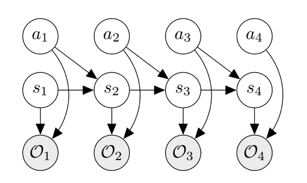
Hidden Markov Models
A HMM
- the probability of a particular
statedepends only on the previous state:$$Pr(q_i\mid q_1, \dots, q_{i-1}) = Pr(q_i \mid q_{i-1});$$ - the probability of an
output observation$o_i$ depends only on the state that produced the observation$q_i$ and not on any other states or any other observations:$$Pr(o_i\mid q_1, \dots, q_{i-1}, o_1, \cdots, o_{i-1}) = Pr(o_i \mid q_{i}).$$
A HMM model is defined by :
- the vector of initial probabilities
$\pi = [ {\pi}_1, ... {\pi}_q ]$ where$\pi_i = Pr(q_1 = i)$ . - a transition matrix for unobserved sequence
${A}$ :$A = [a_{ij}] = Pr(q_t = j \mid q_{t-1} = i)$ . - a matrix of the probabilities of the observations:
$B = [b_{ki}] = Pr(o_t = s_k \mid q_t = i)$ .
The hidden Markov models should be characterized by three fundamental problems:
- (Likelihood): Given an HMM
$\lambda = (A,B)$ and an observation sequence${O}$ , determine the likelihood$Pr(O|\lambda)$ . - (Decoding): Given an observation sequence
${O}$ and an HMM$\lambda = (A,B)$ , discover the best hidden state sequence${Q}$ . - (Learning): Given an observation sequence
${O}$ and the set of states in the HMM, learn the HMM parameters${A}$ and${B}$ .
- Hidden Markov Model (HMM) Markov Processes and HMM
- 漫谈 Hidden Markov Model
- https://www.maths.lancs.ac.uk/~fearnhea/GTP/
- https://web.stanford.edu/~jurafsky/slp3/A.pdf
- https://pomegranate.readthedocs.io/en/latest/index.html
- http://www.shuang0420.com/2016/11/26/Hidden-Markov-Models/
$$ Pr(O|\lambda)=\prod_{i}\underbrace{Pr(o_i \mid q_{i})}{observed} \underbrace{Pr(q_i\mid \lambda)}{hidden}\ = \sum_{i}Pr(O, q_i\mid \lambda) $$
The forward algorithm
Forward probability is defined as
- Initialization:
$\alpha_1(i)=Pr(o_1, q_1=i\mid \lambda)=\pi_i Pr(o_1\mid q_1=i)=\pi_1 b_{o_1i}\quad\forall i$ ; - Recursion:
$\alpha_t(i)=[\sum_{j}\alpha_{t-1}(j)a_{ji}]b_{o_ti}\quad\forall i$ ; - Termination:
$Pr(O\mid \lambda)=\sum_{i}\alpha_T(i)$ .
The backward algorithm
Backward probability is defined as
- Initialization:
$\beta_T(i)=1,\quad i=1,2,\cdots,N$ ; - For
$t=T-1, T-2,\cdots, 1$ ,$$\beta_t(i)=\sum_{j=1}^Na_{ij}b_j(o_{t+1})\beta_{t+1}(j),\quad i=1,2,\cdots,N$$ - Termination:
$Pr(O\mid \lambda)=\sum_{i}\pi_i b_i(o_1)\beta_1(i)$ .
- https://www.wikiwand.com/en/Forward_algorithm
- https://www.wikiwand.com/en/Forward–backward_algorithm
Given an HMM
Viterbi is a kind of dynamic programming Viterbi algorithm
that makes uses of a dynamic programming trellis.
Given an observation sequence
Baum-Welch Algorithm
Baum-Welch Algorithm is exactly an application of expectation maximum algorithm.
The Q function is defined as
As usual, the key step of expectation maximum is to find the
- https://www.wikiwand.com/en/Baum%E2%80%93Welch_algorithm
- http://www.cs.jhu.edu/~jason/papers/#eisner-2002-tnlp
- http://www.kanungo.com/software/software.html#umdhmm
- http://pandamatak.com/people/anand/771/html/node26.html
Probabilistic graphical models provide a formal lingua franca for modeling and a common target for efficient inference algorithms. Their introduction gave rise to an extensive body of work in machine learning, statistics, robotics, vision, biology, neuroscience, artificial intelligence (AI) and cognitive science. However, many of the most innovative and useful probabilistic models published by the AI, machine learning, and statistics community far outstrip the representational capacity of graphical models and associated inference techniques. Models are communicated using a mix of natural language, pseudo code, and mathematical formulae and solved using special purpose, one-off inference methods. Rather than precise specifications suitable for automatic inference, graphical models typically serve as coarse, high-level descriptions, eliding critical aspects such as fine-grained independence, abstraction and recursion.
PROBABILISTIC PROGRAMMING LANGUAGES aim to close this representational gap, unifying general purpose programming with probabilistic modeling; literally, users specify a probabilistic model in its entirety (e.g., by writing code that generates a sample from the joint distribution) and inference follows automatically given the specification. These languages provide the full power of modern programming languages for describing complex distributions, and can enable reuse of libraries of models, support interactive modeling and formal verification, and provide a much-needed abstraction barrier to foster generic, efficient inference in universal model classes.
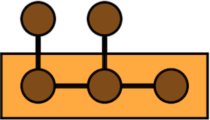
| Graph Nets library |
|---|
 |
| There is a list of existing probabilistic programming systems at http://www.probabilistic-programming.org/wiki/Home and a list of research articles on probabilistic programming until 2015. |
The Algorithms Behind Probabilistic Programming includes: Bayesian Inference, Hamiltonian Monte Carlo and the No U-Turn Sampler, Variational Inference and Automatic Differentation and Probabilistic Programming Languages.
- Graph Nets library
- Hakaru a simply-typed probabilistic programming language
- PROBPROG 2018 -- The International Conference on Probabilistic Programming
- PyMC: Probabilistic Programming in Python
- Stan: a platform for statistical modeling and high-performance statistical computation.
- Welcome to Pyro Examples and Tutorials!
- Edward, and some motivations
- Monadic probabilistic programming in Scala with Rainier
- Factorie: a toolkit for deployable probabilistic modeling, implemented as a software library in Scala
- InferPy: Probabilistic Modeling with Tensorflow Made Easy
- GluonTS - Probabilistic Time Series Modeling
- BTYDplus: Probabilistic Models for Assessing and Predicting your Customer Base
- A Simple Embedded Probabilistic Programming Language
- A modern model checker for probabilistic systems
- emcee: Seriously Kick-Ass MCMC
- Gen: MIT probabilistic programming language
- Probabilistic Programming Primer
- PROBABILISTIC-PROGRAMMING.org
- Programming Languages and Logics Fall 2018
- CAREER: Blending Deep Reinforcement Learning and Probabilistic Programming
- Inference for Probabilistic Programs: A Symbolic Approach
- CSCI E-82A Probabilistic Programming and Artificial Intelligence Stephen Elston, PhD, Principle Consultant, Quantia Analytics LLC
- MIT Probabilistic Computing Project
- Beast2: Bayesian evolutionary analysis by sampling teee
- 36-402, Undergraduate Advanced Data Analysis, Section A
- Machine Learning
- HiPEDS Seminar: Probabilistic models and principled decision making @ PROWLER.io
- Probabilistic Model-Based Reinforcement Learning Using The Differentiable Neural Computer
- Probabilistic Modeling and Inference
- MIT Probabilistic Computing Project


