random_variables_20191111_152_chang.Rmd

---
title: "R Notebook"
output: html_notebook
---

# Chapter 14 Random variables

In data science, we often deal with data that is affected by chance in some way: the data comes from a random sample, the data is affected by measurement error, or the data measures some outcome that is random in nature. __Being able to quantify the uncertainty introduced by randomness is one of the most important jobs of a data analyst.__ Statistical inference offers a framework, as well as several practical tools, for doing this. The first step is to learn how to mathematically describe random variables.

In this chapter, we introduce random variables and their properties starting with their application to games of chance. We then describe some of the events surrounding the financial crisis of 2007-2008 using probability theory. This financial crisis was in part caused by underestimating the risk of certain securities sold by financial institutions. Specifically, the risks of mortgage-backed securities (MBS) and collateralized debt obligations (CDO) were grossly underestimated. These assets were sold at prices that assumed most homeowners would make their monthly payments, and the probability of this not occurring was calculated as being low. A combination of factors resulted in many more defaults than were expected, which led to a price crash of these securities. As a consequence, banks lost so much money that they needed government bailouts to avoid closing down completely.

## 14.1 Random variables

Random variables are numeric outcomes resulting from random processes. We can easily generate random variables using some of the simple examples we have shown. For example, define `X` to be 1 if a bead is blue and red otherwise:
```{r}
beads<-rep(c("red","blue"), times=c(2,3))
x<-ifelse(sample(beads, 1)=="blue", 1, 0)
```
Here `X` is a random variable: every time we select a new bead the outcome changes randomly. See below:
```{r}
ifelse(sample(beads, 1)=="blue",1,0)
ifelse(sample(beads, 1)=="blue",1,0)
ifelse(sample(beads, 1)=="blue",1,0)
```

Sometimes it’s 1 and sometimes it’s 0.

## 14.2 Sampling models

Many data generation procedures, those that produce the data we study, can be modeled quite well as draws from an urn. For instance, we can model the process of polling likely voters as drawing 0s (Republicans) and 1s (Democrats) from an urn containing the 0 and 1 code for all likely voters. In epidemiological studies, we often assume that the subjects in our study are a random sample from the population of interest. The data related to a specific outcome can be modeled as a random sample from an urn containing the outcome for the entire population of interest. Similarly, in experimental research, we often assume that the individual organisms we are studying, for example worms, flies, or mice, are a random sample from a larger population. Randomized experiments can also be modeled by draws from an urn given the way individuals are assigned into groups: when getting assigned, you draw your group at random. Sampling models are therefore ubiquitous in data science. Casino games offer a plethora of examples of real-world situations in which sampling models are used to answer specific questions. We will therefore start with such examples.

Suppose a very small casino hires you to consult on whether they should set up roulette wheels. To keep the example simple, we will assume that 1,000 people will play and that the only game you can play on the roulette wheel is to bet on red or black. The casino wants you to predict how much money they will make or lose. They want a range of values and, in particular, they want to know what’s the chance of losing money. If this probability is too high, they will pass on installing roulette wheels.

We are going to define a random variable $S$ that will represent the casino’s total winnings. Let’s start by constructing the urn. A roulette wheel has 18 red pockets, 18 black pockets and 2 green ones. So playing a color in one game of roulette is equivalent to drawing from this urn:
```{r}
color<-rep(c("Black","Red","Green"), c(18,18,2))
```

The 1,000 outcomes from 1,000 people playing are independent draws from this urn. If red comes up, the gambler wins and the casino loses a dollar, so we draw a -1 dollar. Otherwise, the casino wins a dollar and we draw a 1 dollar. To construct our random variable $S$, we can use this code:
```{r}
n<-1000
X<-sample(ifelse(color=="Red",-1,1), n, replace=TRUE)
X[1:10]
```
Because we know the proportions of 1s and -1s, we can generate the draws with one line of code, without defining `color`:
```{r}
X<-sample(c(-1,1), n, replace=TRUE, prob=c(9/19, 10/19))
```
We call this a sampling model since we are modeling the random behavior of roulette with the sampling of draws from an urn. The total winnings $S$ is simply the sum of these 1,000 independent draws:
```{r}
X<-sample(c(-1,1), n, replace=TRUE, prob=c(9/19, 10/19))
S<-sum(X)
S
```

## 14.3 The probability distribution of a random variable

If you run the code above, you see that $S$ changes every time. This is, of course, because $S$ is a random variable. The probability distribution of a random variable tells us the probability of the observed value falling at any given interval. So, for example, if we want to know the probability that we lose money, we are asking the probability that $S$ is in the interval $S<0$.

Note that if we can define a cumulative distribution function $F(a)=Pr(S<=a)$, then we will be able to answer any question related to the probability of events defined by our random variable $S$, including the event $S<0$. We call this $F$ the random variable’s _distribution function_.

We can estimate the distribution function for the random variable $S$ by using a Monte Carlo simulation to generate many realizations of the random variable. With this code, we run the experiment of having 1,000 people play roulette, over and over, specifically $B=10,000$ times:
```{r}
n<-1000
B<-10000
roulette_winnings <- function(n){
  X<-sample(c(-1,1), n, replace=TRUE, prob=c(9/19,10/19))
  sum(X)
}
S<-replicate(B,roulette_winnings(n))
```
  
Now we can ask the following: in our simulations, how often did we get sums less than or equal to `a`?
```{r}
mean(S<=a)
```
This will be a very good approximation of $F(a)$ and we can easily answer the casino’s question: how likely is it that we will lose money? We can see it is quite low:
```{r}
mean(S<0)
```
We can visualize the distribution of $S$ by creating a histogram showing the probability $F(a)-F(b)$ for several intervals (a,b].

![histogram](https://rafalab.github.io/dsbook/book_files/figure-html/normal-approximates-distribution-1.png)
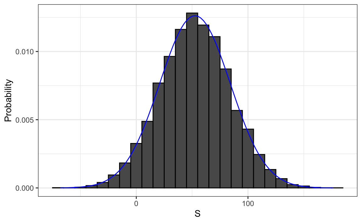
We see that the distribution appears to be approximately normal. A qq-plot will confirm that the normal approximation is close to a perfect approximation for this distribution. If, in fact, the distribution is normal, then all we need to define the distribution is the average and the standard deviation. Because we have the original values from which the distribution is created, we can easily compute these with `mean(S)` and `sd(S)`. The blue curve you see added to the histogram above is a normal density with this average and standard deviation.

This average and this standard deviation have special names. They are referred to as the _expected value_ and _standard error_ of the random variable $S$.

Statistical theory provides a way to derive the distribution of random variables defined as independent random draws from an urn. Specifically, in our example above, we can show that $(S+n)/2$ follows a binomial distribution. We therefore do not need to run for Monte Carlo simulations to know the probability distribution of $S$. We did this for illustrative purposes.

We can use the function `dbinom` and `pbinom` to compute the probabilities exactly. For example, to compute $Pr(S<0)$ we note that:
$$
Pr(S<0)=Pr((S+n)/2 < (0+n)/2)
$$
and we can use the `pbinom` to compute
$$
Pr(S \leq 0)
$$

```{r}
n<-1000
pbinom(n/2, size=n, prob=10/19)
```
Because this is a discrete probability function, to get $Pr(S<0)$ rather than $Pr(S\leq 0)$, we write:
```{r}
pbinom(n/2-1, size=n, prob=10/19)
```
Here we do not cover these details. Instead, we will discuss an incredibly useful approximation provided by mathematical theory that applies generally to sums and averages of draws from any urn: the Central Limit Theorem (CLT).

## 14.4 Distributions versus probability distributions

Before we continue, let’s make an important distinction and connection between the distribution of a list of numbers and a probability distribution. In the visualization chapter, we described how any list of numbers $x1,…,xn$ has a distribution. The definition is quite straightforward. We define $F(a)$ as the function that tells us what proportion of the list is less than or equal to $a$. Because they are useful summaries when the distribution is approximately normal, we define the average and standard deviation. These are defined with a straightforward operation of the vector containing the list of numbers `x`:
```{r}
m<-sum(x)/length(x)
s<-sqrt(sum((x-m)^2) / length(x))
```

A random variable $X$ has a distribution function. To define this, we do not need a list of numbers. It is a theoretical concept. In this case, we define the distribution as the $F(a)$ that answers the question: what is the probability that $X$ is less than or equal to $a$? There is no list of numbers.

However, if $X$ is defined by drawing from an urn with numbers in it, then there is a list: the list of numbers inside the urn. In this case, the distribution of that list is the probability distribution of $X$ and the average and standard deviation of that list are the expected value and standard error of the random variable.

Another way to think about it that does not involve an urn is to run a Monte Carlo simulation and generate a very large list of outcomes of $X$. These outcomes are a list of numbers. The distribution of this list will be a very good approximation of the probability distribution of $X$. The longer the list, the better the approximation. The average and standard deviation of this list will approximate the expected value and standard error of the random variable.

## 14.5 Notation for random variables

In statistical textbooks, upper case letters are used to denote random variables and we follow this convention here. Lower case letters are used for observed values. You will see some notation that includes both. For example, you will see events defined as $X≤x$. Here $X$ is a random variable, making it a random event, and $x$ is an arbitrary value and not random. So, for example, $X$ might represent the number on a die roll and $x$ will represent an actual value we see 1, 2, 3, 4, 5, or 6. So in this case, the probability of $X=x$ is 1/6 regardless of the observed value $x$. This notation is a bit strange because, when we ask questions about probability, $X$ is not an observed quantity. Instead, it’s a random quantity that we will see in the future. We can talk about what we expect it to be, what values are probable, but not what it is. But once we have data, we do see a realization of $X$. So data scientists talk of what could have been after we see what actually happened.

## 14.6 The expected value and standard error

We have described sampling models for draws. We will now go over the mathematical theory that lets us approximate the probability distributions for the sum of draws. Once we do this, we will be able to help the casino predict how much money they will make. The same approach we use for the sum of draws will be useful for describing the distribution of averages and proportion which we will need to understand how polls work.

The first important concept to learn is the expected value. In statistics books, it is common to use letter `E` like this:
$$
E[X]
$$
to denote the expected value of the random variable `X`.

A random variable will vary around its expected value in a way that if you take the average of many, many draws, the average of the draws will approximate the expected value, getting closer and closer the more draws you take.

Theoretical statistics provides techniques that facilitate the calculation of expected values in different circumstances. For example, a useful formula tells us that the expected value of a random variable defined by one draw is the average of the numbers in the urn. In the urn used to model betting on red in roulette, we have 20 one dollars and 18 negative one dollars. The expected value is thus:
$$
E[X]=(20+-18)/38
$$
which is about 5 cents. It is a bit counterintuitive to say that `X` varies around 0.05, when the only values it takes is 1 and -1. One way to make sense of the expected value in this context is by realizing that if we play the game over and over, the casino wins, on average, 5 cents per game. A Monte Carlo simulation confirms this:
```{r}
B <- 10^6
x <- sample(c(-1,1), B, replace = TRUE, prob=c(9/19, 10/19))
mean(x)
```
In general, if the urn has two possible outcomes, say a and b, with proportions p and 1−p respectively, the average is:
$$
E[X]=ap+b(1-p)
$$
To see this, notice that if there are n beads in the urn, then we have $npa$s and $n(1−p)b$s and because the average is the sum, $n*a*p+n*b*(1-p)$, To see this, divided by the total n, we get that the average is $ap+b(1-p)$.

Now the reason we define the expected value is because this mathematical definition turns out to be useful for approximating the probability distributions of sum, which then is useful for describing the distribution of averages and proportions. The first useful fact is that the expected value of the sum of the draws is:
__number of draws * average of the numbers in the urn__

So if 1,000 people play roulette, the casino expects to win, on average, about 1,000 * 0.05 dollars = 50 dollars. But this is an expected value. How different can one observation be from the expected value? The casino really needs to know this. What is the range of possibilities? If negative numbers are too likely, they will not install roulette wheels. Statistical theory once again answers this question. The standard error (SE) gives us an idea of the size of the variation around the expected value. In statistics books, it’s common to use:
$$
SE[X]
$$
to denote the standard error of a random variable.

__If our draws are independent__, then the standard error of the sum is given by the equation:
__sqrt(number of draws) * standard deviation of the numbers in the urn__

Using the definition of standard deviation, we can derive, with a bit of math, that if an urn contains two values a and b with proportions p and (1−p), respectively, the standard deviation is:
$$
|b-a|\sqrt{p(1 - p)}
$$
So in our roulette example, the standard deviation of the values inside the urn is:
$|1 - (-1)|\sqrt{10/19\times9/19}$ or:
```{r}
2*sqrt(90)/19
```

The standard error tells us the typical difference between a random variable and its expectation. Since one draw is obviously the sum of just one draw, we can use the formula above to calculate that the random variable defined by one draw has an expected value of 0.05 and a standard error of about 1. This makes sense since we either get 1 or -1, with 1 slightly favored over -1.

Using the formula above, the sum of 1,000 people playing has standard error of about $32:
```{r}
n<-1000
sqrt(n)*2*sqrt(90)/19
```
As a result, when 1,000 people bet on red, the casino is expected to win $50 with a standard error of $32. It therefore seems like a safe bet. But we still haven’t answered the question: how likely is it to lose money? Here the CLT will help.

Advanced note: Before continuing we should point out that exact probability calculations for the casino winnings can be performed with the binomial distribution. However, here we focus on the CLT, which can be generally applied to sums of random variables in a way that the binomial distribution can’t.

### 14.6.1 Population SD versus the sample SD

The standard deviation of a list `x` (below we use heights as an example) is defined as the square root of the average of the squared differences:
```{r}
library(dslabs)
x <- heights$height
m <- mean(x)
s <- sqrt(mean((x-m)^2))
```
Using mathematical notation we write:
$$
\mu = \frac{1}{n} \sum_{i=1}^n x_i \\
\sigma =  \sqrt{\frac{1}{n} \sum_{i=1}^n (x_i - \mu)^2}
$$
However, be aware that the `sd` function returns a slightly different result:
```{r}
identical(s,sd(x))
s-sd(x)
```

This is because the sd function R does not return the sd of the list, but rather uses a formula that estimates standard deviations of a population from a random sample $X_1,...,X_N$ which, for reasons not discussed here, divide the sum of squares by the $N-1$.
$$
\bar{X} = \frac{1}{N} \sum_{i=1}^N X_i, \,\,\,\,
s =  \sqrt{\frac{1}{N-1} \sum_{i=1}^N (X_i - \bar{X})^2}
$$
You can see that this is the case by typing:
```{r}
n <- length(x)
s-sd(x)*sqrt((n-1) / n)
```
For all the theory discussed here, you need to compute the actual standard deviation as defined:
```{r}
sqrt(mean((x-m)^2))
```
So be careful when using the `sd` function in R. However, keep in mind that throughout the book we sometimes use the `sd` function when we really want the actual SD. This is because when the list size is big, these two are practically equivalent since $\sqrt{(N-1)/N} \approx 1$.