statistical_inference_20191120_152_chang.Rmd

---
title: "R Notebook"
output: html_notebook
---

# Chapter 15 Statistical inference

## 15.1 Polls

Inference: statistical theory to justify the strategy of interviewing random smaller group and infer the opinions of the entire population.

MoE: margin of error

What we will learn: estimates, MoE -> confidence, p-value->Bayesian modeling->apply

### 15.1.1 The sampling model of polls

Let's mimic the challenge real pollsters face. The challenge is to guess the spread between the proportion of blue and red beads in the urn. 25 dollars for winner. It costs 0.1 dollars per each bead sampling.

1st phase: if the interval you submit contains the true proportion, you get half what you paid and pass to the second phase

2nd phase: entry with samllest interval is the winner

```{r}
library(tidyverse)
library(dslabs)
take_poll(25)
```
Red: Republican
Blue: Democrats
->only 2 parties

## 15.2 Populations, samples, parameters, and estimates

proportion of blue beeds: p
proportion of red beeds: 1-p
spread: p-(1-p) = 2p-1

beads: population
p: parameter
25 beads: sample

inference: predict p using observed data in the sample

### 15.2.1 The sample average

random variable X: 
  X=1 represents a blue bead
  X=0 represents a red bead

->adding Xs is counting blue beads
->dividing by N is computing a proportion
-->average $\bar{X}$
$$
\bar{X} = 1/N \times \sum_{i=1}^N X_i
$$
What we are going to do: estimate p

### 15.2.2 Parameters

in statistical inference we define __parameters__ to define unknown parts of our models.

### 15.2.3 Polling versus forecasting

The p for election night might be different from a poll conducted before since people’s opinions fluctuate through time.

### 15.2.4 Properties of our estimate: expected value and standard error

the expected value of the average $\bar{X}$ is $p$
$$
E(\bar{X}) = p
$$
standard error of the sum is $\sqrt{N} \times$ the standard deviation of the urn
$$
SE(\bar{X}) = \sqrt{p(1-p)/N}
$$
we can make the standard error as small as we want by increasing N.
__The law of large numbers__ tells us that with a large enough poll, our estimate converges to  
p.

let’s assume that $p=0.51$ and make a plot of the standard error versus the sample size N:

![plot](https://rafalab.github.io/dsbook/book_files/figure-html/standard-error-versus-sample-size-1.png)

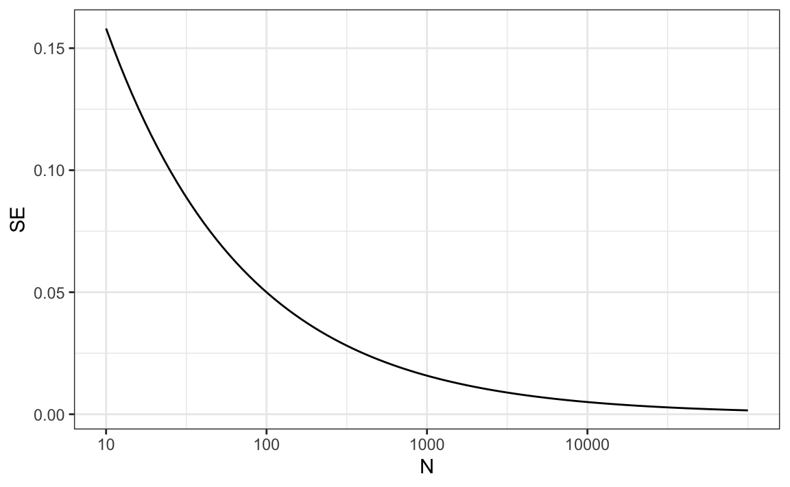
we would need a poll of over 10,000 people to get the standard error 1%

For a sample size of 1,000 and $p=0.51$, the standard error is:
```{r}
p=0.51
sqrt(p*(1-p))/sqrt(1000)
```

## 15.3 Exercises

1. 25p
2. sqrt(25p(1-p))
3. p
4. sqrt(p(1-p)/25)
5. 
```{r}
p<-seq(0, 1, length = 100)
se<-sqrt(p*(1-p)/25)
plot(p,se)
```

6. 
```{r}
for(n in c(25, 100, 1000)){
  se<-sqrt(p*(1-p)/n)
plot(p,se)
}
```
7. $\mbox{E}(d)=\mbox{E}(\bar{X}−(1−\bar{X}))=\mbox{E}(2\bar{X}−1) =2\mbox{E}(\bar{X})−1 =2p−1=p−(1−p)$

8.$\mbox{SE}(d)=\mbox{SE}[\bar{X}−(1−\bar{X})]=\mbox{SE}[2\bar{X}−1] =2\mbox{SE}[\bar{X}] =2\sqrt{p(1−p)/N}$

9. 
```{r}
p<-0.45
2*sqrt(p*(1-p)/25)
```
10. Given the answer to 9, which of the following best describes your strategy of using a sample size of N=25?
b. Our standard error is larger than the difference, so the chances of 2$\bar{X}$−1 being positive and throwing us off were not that small. We should pick a larger sample size.

## 15.4 Central Limit Theorem in practice

distribution function for a sum of draws is approximately normal. 
dividing a normally distributed random variable by a constant is also a normally distributed variable.
->$\bar{X}$ has an approximately normal distribution
expected value: p
standard error: $\sqrt{p(1-p)/N}$

what is the probability that we are within 1% from p?
<=>$\mbox{Pr}(| \bar{X} - p| \leq .01)$
<=>$\mbox{Pr}(\bar{X}\leq p + .01) - \mbox{Pr}(\bar{X} \leq p - .01)$

making this to standard normal random variable
$$
\mbox{Pr}\left(Z \leq \frac{ \,.01} {\mbox{SE}(\bar{X})} \right) -
\mbox{Pr}\left(Z \leq - \frac{ \,.01} {\mbox{SE}(\bar{X})} \right) 
$$
$\mbox{SE}(\bar{X}) = \sqrt{p(1-p)/N}$

even though we do not know p, we plug-in the estimate with $\bar{X}$

$$
\hat{\mbox{SE}}(\bar{X})=\sqrt{\bar{X}(1-\bar{X})/N}
$$
hat means estimates

In our first sample we had 12 blue and 13 red -> $\bar{X}=0.48$
estimate of standard error is:
```{r}
x_hat<-0.48
se<-sqrt(x_hat*(1-x_hat)/25)
se
```
now we can answer the question of the probability of being close to p. The answer is:
```{r}
pnorm(0.01/se)-pnorm(-0.01/se)
```
N=25 is not enough

margin of error = two times the standard error
```{r}
1.96*se
```
why 1.96?
```{r}
pnorm(1.96)-pnorm(-1.96)
```
there is a 95% probability that $\bar{X}$ will be within $1.96 \times \hat{SE}(\bar{X})$

### 15.4.1 A Monte Carlo simulation

Monte Carlo simulation to corroborate the tools we have built using probability theory
```{r}
B<-10000
N<-1000
x_hat<-replicate(B,{
  x<-sample(c(0,1), size=N, replace=TRUE, prob=c(1-p,p))
  mean(x)
})
```
the problem is that we do not know p. pick several values of p. let's set p=0.45
```{r}
p<-0.45
N<-1000
x<-sample(c(0,1), size=N, replace=TRUE, prob=c(1-p,p))
x_hat<-mean(x)
```
our estimate is `x_hat`.
```{r}
B <- 10000
x_hat <- replicate(B, {
  x <- sample(c(0,1), size = N, replace = TRUE, prob = c(1-p, p))
  mean(x)
})
```

$\bar{X}$ is approximately normally distributed, has expected value p=0.45 and se=$\sqrt{p(1-p)/N}=0.016$
the simulation confirms this
```{r}
mean(x_hat)
sd(x_hat)
```
A histogram and qq-plot confirm that the normal approximation is accurate as well:
![histqq](https://rafalab.github.io/dsbook/book_files/figure-html/normal-approximation-for-polls-1.png)

### 15.4.2 The spread

the spread is 2p-1.
our estimate $\bar{X}$ and $\hat{SE}(\bar{X})$
-> spread: $2\bar{X}-1$
standard error: $2\hat{SE}(\bar{X})$

### 15.4.3 Bias: why not run a very large poll?

1. too many samplings are expensive
2. theory has limitations ->bias:even if our margin of error is very small, it might not be exactly right that our expected value is p

## 15.5 Exercising

1. 
```{r}
take_sample<-function(p,N){
  X <- sample(c(0,1), size = N, replace = TRUE, prob = c(1-p, p))
  mean(X)
}
```

2. 
```{r}
p<-0.45
N<-100
errors<-replicate(10000, take_sample(p,N)-p)
```

3. 
```{r}
mean(errors)
hist(errors)
```
c. The errors are symmetrically distributed around 0.

4. 
```{r}
mean(abs(errors))
```

5. 
```{r}
sd(errors)
```

6. 
```{r}
sqrt(p*(1-p)/100)
```

7. 
```{r}
set.seed(1)
X<-sample(c(0,1), size = N, replace = TRUE, prob = c(1-p, p))
X_bar = mean(X)
sqrt(X_bar*(1-X_bar)/N)
```
Note how close the standard error estimates obtained from the Monte Carlo simulation (exercise 5), the theoretical prediction (exercise 6), and the estimate of the theoretical prediction (exercise 7) are. 

8. 
```{r}
library(tidyverse)
library(ggplot2)
p<-0.5
N<-seq(100,5000,100)
se<-sqrt(p*(1-p)/N)
df<-data.frame(N,se)
df %>% ggplot(aes(N,se)) + geom_line()
```
how large does the sample size have to be to have a standard error of about 1%?

c. 2500

9. For sample size N=100, the central limit theorem tells us that the distribution of $\bar{X}$ is:

b. approximately normal with expected value p and standard error $\sqrt{p(1-p)/N}$

10.  the error $\bar{X}-p$ is:

b. approximately normal with expected value 0 and standard error $\sqrt{p(1-p)/N}$

11. 
```{r}
qqnorm(errors)
qqline(errors)
```

12.
```{r}
p<-0.45
N<-100
1-pnorm(0.5, p, sqrt(p*(1-p)/N))
```

13.
```{r}
se<-sqrt(0.51*(1-0.51)/100)
1-pnorm(0.01,0,se)
```