Project description: Using data from the fictitious Power City, the goal of this research is to construct predictive models for electrical energy production from wind and solar sources, and energy consumption across eight city sectors that can effectively forecast at an hourly level. My team also forecasted production and consumption values for a diverse set of days over the course of a single scenario year. Ultimately, these models can be used to assist in planning the demand-supply of renewable energy for a single city. Multiple machine learning methods (time series, neural networks, boosting, decision trees, random forest, and support vector machines) were explored and their performances were compared across ten datasets: wind and solar energy production, and consumption for eight sectors.
The data used for this project originated from fourteen files of raw data regarding Power City's energy production and consumption. All production and consumption files include hourly data – twenty-four records per day. Weather conditions and calendar specifics between all files include:
- Weather Condition Features: solar elevation, cloud cover, dew point, humidity, precipitable water, temperature, visibility, wind speed, and pressure
- Calendar Day Features: day of the week, holiday, school day
In order to get the files into a more comprehensible and cohesive format, some preliminary features were added and others were normalized in order to merge files. Initially separated time varibles (day, month, hour) were combined to generate a single DateTime column.
from datetime import datetime

powercity_weather_consumption['Date_Time_Stamp'] = pd.to_datetime(dict(year=2015,
                                                                       month=powercity_weather_consumption['Month'],
                                                                       day=powercity_weather_consumption['Day'],
                                                                       hour=powercity_weather_consumption['Hour']))
Only two files had missing data: the scenario year weather and the solar array weather. Most of the missing values were filled in using the median value of the two weeks preceding and following the missing data point (median was preferred over mean due to the count of zeros in the data). The only exception was filling in values for Precipitation and Pressure variables, since many consecutive values were missing; for those values, the average of previous years was used to complete the data.
#replace missing values for Cloud_Cover_Fraction using the median value of the two weeks preceding and following the missing data point
rows = len(powercity_weather_scenario)

for i in range(rows):
    val = powercity_weather_scenario.loc[i][5]
    #print(val)
    if np.isnan(val):
        #print(val)
        powercity_weather_scenario['Cloud_Cover_Fraction'] = powercity_weather_scenario['Cloud_Cover_Fraction'].replace(powercity_weather_scenario['Cloud_Cover_Fraction'][i],
                                                                                                                        powercity_weather_scenario['Cloud_Cover_Fraction'][i-336:i+336].median())
Once the files were merged, each was aggregated (using mean) by day to simplify the problem and smooth some of the noise coming from the weather data. The consumption data was subset into eight separate files, each representing a single sector of usage (residential, K-12 schools, etc.).
consump_fs = consump[consump.Sector == 'FOOD_SERVICE']
consump_g = consump[consump.Sector == 'GROCERY']
consump_hc = consump[consump.Sector == 'HEALTH_CARE']
consump_k12 = consump[consump.Sector == 'K12_SCHOOLS']
consump_l = consump[consump.Sector == 'LODGING']
consump_o = consump[consump.Sector == 'OFFICE']
consump_r = consump[consump.Sector == 'RESIDENTIAL']
consump_sar = consump[consump.Sector == 'STAND_ALONE_RETAIL']
Feature engineering was used to create additional calendar variables (such as ‘Weekend’ and ‘Season’), and dummy variables were extracted from categorical variables (‘Month’, ‘Day’, ‘Day of week’). All files except for the scenario file were split into 80/20 train/test sets. Below is a summary table of the main four(4) aggregated datasets and their corresponding features.

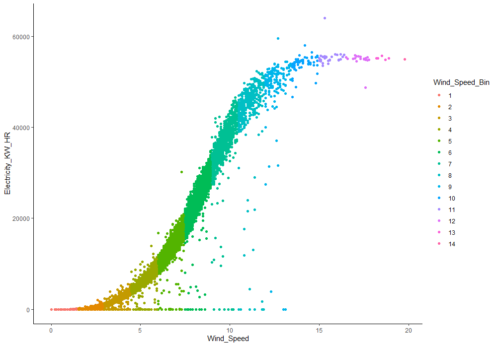
In observing the wind data, a nearly perfect linear relationship can be seen between wind speed and electricity production, which is no surprise; the greater the speed of the wind, the higher the production of electricity (Figure: Electricity Production by Wind Speed). However, from the plot, the level of energy starts to plateau after wind energy reaches a certain high level.
Initial exploratory analysis was done in RStudio to identify starting autoregression, moving average, seasonality, and other parameters. Indepedent variable (electricity consumed) was tested for normality. Using the ACF, PACF, and EACF plots, potential seasonal parameters were identified, and also validated using the auto.arima() function. Models were then constructed using the SARIMAX() function from Python statsmodels library. The best performing parameters from the analysis done in RStudio were used to construct models, and the exogenous variables were reintroduced (weather conditions, calendar day features, etc.). The models were then tested against a test set using the RMSE and explained variance scores for evaluation. The parameters of each model were tweaked until the highest performing model was produced.
Based on the low explained variance, models built for a couple of sectors (food service, residential) were considered unsuccessful. This might be due to limited data (one year worth) of city sectors' electricity consumption, while consumption appeared to be highly volatile during summer months.


A multilinear regression algorithm was explored for model creation, using the LinearRegression function in Sci-Kit Learn. RMSE and R-Square were used for evaluating the model performance. Overall, these models performed decently well but much worse than other algorithms which might indicate that nonlinear models could fit these datasets better; so further tuning of these models were halted
Initially, artificial neural networks were trained using the three consolidated datasets: wind production, solar production, and consumption. After reviewing and taking into consideration the different consumption patterns of eight sectors, ANNs were then trained on the ten datasets. Recurrent neural networks (RNN) and long-short term memory models (LSTM) on Keras were trained and tuned. An additional pre-processing step to prepare the training data frame was applied: turning time series data into supervised data frame. More specifically, in this project, RNN and LSTM use a twenty-four-time step, or a day’s worth of data, to learn and ultimately make predictions. The final step applied to training and validation data was to reshape the data frame to have dimensions in the following order: number of samples, time-step size, number of features.
# Reshape train/valid input data to be Keras-ready format [samples, timesteps, features]

x_train = x_train.reshape((x_train.shape[0], 24, 2))
x_valid = x_valid.reshape((x_valid.shape[0], 24, 2))
print(x_train.shape, y_train.shape)
print(x_valid.shape, y_valid.shape)
Training RNN and LSTM models using Keras can be time-consuming due to multiple factors, for example: higher numbers of trainable parameters, or high numbers of training epochs. In an effort to see whether a model is a good fit, the initial trained models were trained with only fifty epochs. Model building and training started out with a simple model of [one input layer, one hidden layer, and one output layer]. The training process continued with adding layers and tuning the parameters, such as the number of nodes in each layer, activation function, loss function, optimizer, and performance metrics.
# design neural net

model = Sequential()
model.add(LSTM(150, return_sequences=True, input_shape=(x_train.shape[1], x_train.shape[2])))
model.add(Dropout(0.2))
model.add(LSTM(300, return_sequences=True))
model.add(Dropout(0.2))
model.add(LSTM(300, return_sequences=False))
model.add(Dropout(0.2))
model.add(Dense(1, activation = 'relu'))  #activations tried: linear, sigmoid, tanh, softmax, relu

model.compile(loss='mse',
              optimizer='adam',
              metrics=['mae'])

model.summary()
#fit neural net

history = model.fit(x_train, y_train,
                    epochs=50,
                    batch_size=30,
                    verbose=2,
                    shuffle=False,
                    validation_data=(x_valid, y_valid))
The model trained with the training set is validated with validation set, by looking at the output of the losses after each training epoch. The lower value of loss (approaching zero) and the faster the loss decreases, the better and faster a neural network model learns. Ideally, the sign of a potential good model is a continuously small gap (low level of oscillation) between the training’s losses and validation’s losses. While LSTM model showed that the losses were decreasing, there was a gap between training’s losses and validation’s losses, and the decrease was slow. RNN was less successful, as the losses shown oscillating pattern. Further effort of training didn’t return any ANN with higher potential. This led the project to make a decision of moving towards using ANNs run by Sci-kit learn. Sci-kit learn neural network function helped make the training process much simpler: data split with randomization of rows, no requirement to convert time series data into supervised data frame, smaller number of parameters to be tuned. Interestingly, the ANNs’ performances showed improvement and potential, but did not show as much success when evaluated against other algorithms experimented in this project.
In the case of decision trees and random forests, the training and fitting of models for wind production, solar production, and consumption were performed on the 10 datasets, where consumption is subset into eight sectors. Using Sci-kit learn, DecisionTreeRegressor and RandomForestRegressor functions are called, and parameters are tuned by Grid search and manually. For decision tree, the following parameters were used: criterion, splitter, min samples split, min samples leaf. Random tree models were also utilized to find features importance in order to reduce features for training ANNs. For random forest, the following parameters were used: n estimators, max features, min samples split. Decision tree models have high RMSE scores across ten datasets, especially for solar production with the second highest RMSE. On the other hand, random forests have some of the best scores for RSME across eight consumption sectors (K-12 schools, lodging, office, residential), as well as solar production.
From building and training random forest models, there was a consistent pattern of good performances based on RMSE and R-squared scores. As a result, random forest was chosen as the main algorithm for all ten datasets, including wind production, solar production, and the eight consumption sectors. As one potential random forest model for each of these datasets was identified, it was further tuned and tested using test sets. Models for wind and solar production were more straightforward, as they are two separate models. However, this is not the case for Consumption sectors, as the project’s objective is to build a model for Power City’s consumption as a whole. The best random forest model identified for each consumption sector had different parameters’ values compared to the other sectors’ best random forest models. In order to provide a more parsimonious solution, all eight sectors’ random forest models were compared and manually tested to find the best combination of parameters for a final model that can maintain or improve predictive performance for each sector’s consumption. In order to evaluate the final random forests model, the predicted value for each calendar day (average of electricity consumption of the day) was calculated by summing up the predicted values of all eight sectors’ consumption on that day. The last step was to use this model and make predictions using scenario dataset. These predictions are used as a tool to demonstrate the functionality of random forest model for Power City’s daily average energy consumption.
As a regression problem, the most common metric to use to evaluate the performance is the RMSE value. This metric indicates if the model can be good at predicting the observed data. Another performance metric to consider is the R2 value. R2 is a statistical measure of how close the data is to the regression line. This also tells how the target variable can be explained by the predictors from the model. Table 5 shows the RMSE and R2 evaluation of the highest performing model constructed by every algorithm on all ten datasets. The highest performing models overall for each data set are highlighted in yellow.

The model had the lowest RMSE value (16,812) and the highest R2 value (0.77) compared to the other models used. The parameters used to create the model required a minimum of six samples before splitting the tree, two-hundred trees, and used the Mean Absolute Error as a criterion to determine the quality of the split. When looking at the model’s feature importance, we found cloud coverage (55.2%), humidity (9.4%), solar elevation (6.8%), dew point (4.7%), and temperature (4.4%) as the top five features from model.
A similar approach was performed to determine the best predictive model for wind energy production. Both AdaBoost and random forest were found to be the best models where they had the same r-squared value (0.98) and a nearly identical RMSE value (1,550 for AdaBoost and 1,558 for random forest). After much consideration which model to choose, the random forest model was chosen since the model for the solar energy production was also a random forest model. The parameters used to create the model required seven samples before splitting the tree and two-hundred trees. The feature importance for this model was only Wind Speed (99%) as the other predictors were dummy variables from feature engineering mentioned previously.