MCMCChains.jl

Implementation of Julia types for summarizing MCMC simulations and utility functions for diagnostics and visualizations.

Example

The following simple example illustrates how to use Chain to visually summarize a MCMC simulation:

using MCMCChains
using StatsPlots

theme(:ggplot2)

# Define the experiment
n_iter = 500
n_name = 3
n_chain = 2

# experiment results
val = randn(n_iter, n_name, n_chain) .+ [1, 2, 3]'
val = hcat(val, rand(1:2, n_iter, 1, n_chain))

# construct a Chains object
chn = Chains(val)

# visualize the MCMC simulation results
p1 = plot(chn)
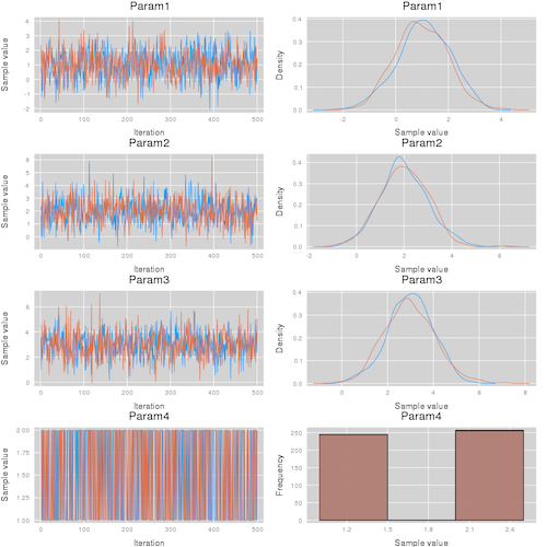
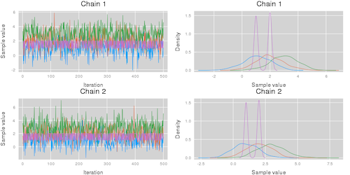
p2 = plot(chn, colordim = :parameter)

This code results in the visualizations shown below. Note that the plot function takes the additional arguments described in the Plots.jl package.

Summarize parameters	Summarize chains
plot(chn; colordim = :chain)	plot(chn; colordim = :parameter)

Manual

Chains type

# construction of a Chains object with no names
Chains(
    val::AbstractArray{A,3};
    start::Int=1,
    thin::Int=1,
    evidence = 0.0,
    info=NamedTuple(),
)

# construction of a chains object with new names
Chains(
    val::AbstractArray{A,3},
    parameter_names::Vector{String},
    name_map = copy(DEFAULT_MAP);
    start::Int=1,
    thin::Int=1,
    evidence = 0.0,
    info=NamedTuple(),
)

# Indexing a Chains object
chn = Chains(...)
chn_param1 = chn[:,2,:] # returns a new Chains object for parameter 2
chn[:,2,:] = ... # set values for parameter 2

Parameter Names

Chains can be constructed with parameter names, like so:

# 500 samples, 5 parameters, two chains.
val = rand(500,5, 2)

chn = Chains(val, ["a", "b", "c", "d", "e"])

By default, parameters will be given the name Parami, where i is the parameter number.

Rename Parameters

Parameter names can be changed with the function set_names, which accepts a Chain object and a Dict containing the mapping between old and new column names. Note that set_names creates a new Chain object because mutation is not supported.

chn = Chains(
	rand(100, 5, 5),
	["one", "two", "three", "four", "five"],
	Dict(:internals => ["four", "five"])
)

# Set "one" and "five" to uppercase.
new_chain = set_names(chn,  Dict(["one" => "ONE", "five" => "FIVE"]))

Sections

Chains parameters are sorted into sections, which are types of parameters. By default, every chain contains a section called :parameters, which is where all values are assigned unless assigned elsewhere. Chains can be assigned a named map during construction:

chn = Chains(val,
  ["a", "b", "c", "d", "e"],
  Dict(:internals => ["d", "e"]))

Or through the set_section function, which returns a new Chains object (as Chains objects cannot be modified in place due to section map immutability):

chn2 = set_section(chn, Dict(:internals => ["d", "e"]))

Any parameters not assigned will be placed into :parameters.

Calling show(chn) provides the following output:

Log evidence      = 0.0
Iterations        = 1:500
Thinning interval = 1
Chains            = 1, 2, 3
Samples per chain = 500
parameters        = c, b, a

Empirical Posterior Estimates
────────────────────────────────────
parameters
   Mean    SD   Naive SE  MCSE  ESS
a 0.5169 0.2920   0.0075 0.0066 500
b 0.4891 0.2929   0.0076 0.0070 500
c 0.5102 0.2840   0.0073 0.0068 500

Quantiles
────────────────────────────────────
parameters
   2.5%   25.0%  50.0%  75.0%  97.5%
a 0.0001 0.2620 0.5314 0.7774 0.9978
b 0.0001 0.2290 0.4972 0.7365 0.9998
c 0.0004 0.2739 0.5137 0.7498 0.9997

Note that only a, b, and c are being shown. You can explicity show the :internals section by calling describe(chn, sections=:internals) or all variables with describe(chn, showall=true). Most MCMCChains functions like plot or gelmandiag support the section and showall keyword arguments.

The get Function

MCMCChains provides a get function designed to make it easier to access parameters get(chn, :P) returns a NamedTuple which can be easy to work with.

Example:

val = rand(500, 5, 1)
chn = Chains(val, ["P[1]", "P[2]", "P[3]", "D", "E"]);

x = get(chn, :P)

Here's what x looks like:

(P = (Union{Missing, Float64}[0.349592; 0.671365; … ; 0.319421; 0.298899], Union{Missing, Float64}[0.757884; 0.720212; … ; 0.471339; 0.5381], Union{Missing, Float64}[0.240626; 0.987814; … ; 0.980652; 0.149805]),)

You can access each of the P[. . .] variables by indexing, using x.P[1], x.P[2], or x.P[3].

get also accepts vectors of things to retrieve, so you can call x = get(chn, [:P, :D]). This looks like

(P = (Union{Missing, Float64}[0.349592; 0.671365; … ; 0.319421; 0.298899], Union{Missing, Float64}[0.757884; 0.720212; … ; 0.471339; 0.5381], Union{Missing, Float64}[0.240626; 0.987814; … ; 0.980652; 0.149805]),
 D = Union{Missing, Float64}[0.648963; 0.0419232; … ; 0.54666; 0.746028])

Note that x.P is a tuple which has to be indexed by the relevant index, while x.D is just a vector.

Convergence Diagnostics functions

Discrete Diagnostic

Options for method are [:weiss, :hangartner, :DARBOOT, MCBOOT, :billinsgley, :billingsleyBOOT]

discretediag(c::Chains; frac=0.3, method=:weiss, nsim=1000)

Gelman, Rubin, and Brooks Diagnostics

gelmandiag(c::Chains; alpha=0.05, mpsrf=false, transform=false)

Geweke Diagnostic

gewekediag(c::Chains; first=0.1, last=0.5, etype=:imse)

Heidelberger and Welch Diagnostics

heideldiag(c::Chains; alpha=0.05, eps=0.1, etype=:imse)

Raftery and Lewis Diagnostic

rafterydiag(c::Chains; q=0.025, r=0.005, s=0.95, eps=0.001)

Model Selection

Deviance Information Criterion (DIC)

chn ... # sampling results
lpfun = function f(chain::Chains) # function to compute the logpdf values
    niter, nparams, nchains = size(chain)
    lp = zeros(niter + nchains) # resulting logpdf values
    for i = 1:nparams
        lp += map(p -> logpdf( ... , x), Array(chain[:,i,:]))
    end
    return lp
end
DIC, pD = dic(chn, lpfun)

Plotting

# construct a plot
plot(c::Chains, seriestype = (:traceplot, :mixeddensity))

# construct trace plots
plot(c::Chains, seriestype = :traceplot)

# or for all seriestypes use the alternative shorthand syntax
traceplot(c::Chains)

# construct running average plots
meanplot(c::Chains)

# construct density plots
density(c::Chains)

# construct histogram plots
histogram(c::Chains)

# construct mixed density plots
mixeddensity(c::Chains)

# construct autocorrelation plots
autocorplot(c::Chains)

# make a cornerplot (requires StatPlots) of parameters in a Chain:
corner(c::Chains, [:A, :B])

Saving and Loading Chains

Chains objects can be serialized and deserialized using read and write.

# Save a chain.
write("chain-file.jls", chn)

# Read a chain.
chn2 = read("chain-file.jls", Chains)

Exporting Chains

A few utility export functions have been provided to convers Chains objects to either an Array or a DataFrame:

# Several examples of creating an Array object:
Array(chns)
Array(chns[:s])
Array(chns, [:parameters])
Array(chns, [:parameters, :internals])

# By default chains are appended. This can be disabled
# using the append_chains keyword argument:
Array(chns, append_chains=false)

# This will return an `Array{Array, 1}` object containing
# an Array for each chain.

# A final option is:
Array(chns, remove_missing_union=false)

# This will not convert the Array columns from a
# `Union{Missing, Real}` to a `Vector{Real}`.

Similarly, for DataFrames:

DataFrame(chns)
DataFrame(chns[:s])
DataFrame(chns, [:parameters])
DataFrame(chns, [:parameters, :internals])
DataFrame(chns, append_chains=false)
DataFrame(chns, remove_missing_union=false)

See also ?DataFrame and ?Array for more help.

Sampling Chains

MCMCChains overloads several sample methods as defined in StatsBase:

# Sampling `n` samples from the chain `a`. Optionally
# weighting the samples using `wv`.
sample([rng], a, [wv::AbstractWeights], n::Integer)

# As above, but supports replacing and ordering.
sample([rng], a, [wv::AbstractWeights], n::Integer; replace=true,
  ordered=false)

See also ?sample for additional help. Alternatively, you can construct and sample from a kernel density estimator using the KernelDensity package:

using KernelDensity

# Construct a kernel density estimator
c = kde(Array(chn[:s]))

# Generate 10000 weighted samples from the grid points
chn_weighted_sample = sample(c.x, Weights(c.density), 100000)

License Notice

Note that this package heavily uses and adapts code from the Mamba.jl package licensed under MIT License, see License.md.