LCA CIFAR Tutorial Part2 Parallel

Introduction

This page is a continuation of the tutorial for using PetaVision and the locally competitive algorithm (LCA) for sparse coding images. The previous page, using LCA to sparse code a single image, is here. On this page, we will see how PetaVision uses MPI for both data parallelism (several images processed in parallel) and model parallelism (one image split across several processes). In the following, make sure that you are in the LCA-CIFAR-Tutorial directory, inside the build directory, that you used in the single-image tutorial. Also make sure that the environment variables PV_SOURCEDIR and PYTHONPATH are defined as before:

$ PV_SOURCEDIR=/path/to/source/OpenPV # change to the correct path on your system
$ export PV_SOURCEDIR
$ export PYTHONPATH="$PYTHONPATH":$PV_SOURCEDIR/python

1. Multiple images

In the preceding run, we sparse coded a single image. The .params file identified this image by setting the parameter inputPath to a single PNG file. We can sparse code several images in a single PetaVision run by setting the input path to a text file containing a list of text files. When we unpacked the CIFAR-10 dataset, we created the cifar-10-images/mixed_cifar.txt file for this purpose.

$ head cifar-10-images/mixed_cifar.txt
cifar-10-images/6/CIFAR_10000.png
cifar-10-images/9/CIFAR_10001.png
cifar-10-images/9/CIFAR_10002.png
cifar-10-images/4/CIFAR_10003.png
cifar-10-images/1/CIFAR_10004.png
cifar-10-images/1/CIFAR_10005.png
cifar-10-images/2/CIFAR_10006.png
cifar-10-images/7/CIFAR_10007.png
cifar-10-images/8/CIFAR_10008.png
cifar-10-images/3/CIFAR_10009.png

To help keep the PetaVision runs straight, we will copy the .lua file to a new file, then edit the new file, and then generate a separate .params file for each run.

$ cp input/LCA_CIFAR.lua input/LCA_CIFAR_Multiple_Images.lua

Then, edit the new .lua file, changing the line

local numImages            = 1;   --Number of images to process.

to

local numImages            = 16;  --Number of images to process.

and the line

local inputPath            "cifar-10-images/6/CIFAR_10000.png"

to

local inputPath            "cifar-10-images/mixed_cifar.txt"

Let's also change the output path so that we can compare the output files of different runs. Change

local outputPath           = "output";

to

local outputPath           = "output_multiple_images";

Then create a .params file and run OpenPV as before. This run will take longer to execute, and the output files will be about 16 times bigger, because we are running for 6400 timesteps instead of 400. However, the run might not take as long as a full 16 times longer, because of initial start up time.

$ lua input/LCA_CIFAR_Multiple_Images.lua > input/LCA_CIFAR_Multiple_Images.params
$ ../tests/BasicSystemTest/Release/BasicSystemTest -p input/LCA_CIFAR_Multiple_Images.params -l LCA-CIFAR-run.log -t 2

We can plot the results of the probes using the pvtools readenergyprobe and readlayerprobe commands, as before. The only difference is that now the directory argument to those commands is the new output_multiple_images directory.

$ python
>>> import pvtools
>>> import matplotlib.pyplot
>>> matplotlib.interactive(True)
>>> matplotlib.pyplot.figure(1)
>>> energydata = pvtools.readenergyprobe(
...   probe_name='TotalEnergyProbe', 
...   directory='output_multiple_images', 
...   batch_element=0)
>>> matplotlib.pyplot.plot(energydata['time'], energydata['values'])
>>> matplotlib.pyplot.title('Total Energy, 16 images, sequential')

Note that the energy value has a spike every 400 timesteps, as a new image arrives, but the sparse coding still corresponds to the old image. The energy then decreases towards a minimum (for that image) as the system solves for the sparse coding of the new image.

Indeed, we can see the reconstruction error spike upward when a new image is presented, and then decrease (but not to zero) as the sparse coding for the new image improves.

>>> matplotlib.pyplot.figure(2)
>>> inputerror = pvtools.readlayerprobe(
...   probe_name='InputErrorL2NormProbe',
...   directory='output_multiple_images',
...   batch_element=0)
>>> matplotlib.pyplot.plot(inputerror['time'], inputerror['values'])

It's worth discussing the values of the sparsity probe in a bit more detail.

>>> matplotlib.pyplot.figure(3)
>>> sparsity = pvtools.readlayerprobe(
...   probe_name='SparsityProbe',
...   directory='output_multiple_images',
...   batch_element=0)
>>> matplotlib.pyplot.plot(sparsity['time'], sparsity['values'])

Note that after the first image, when a new image is presented, the sparsity probe initially decreases, then increases, and then levels off until the next image, when the cycle repeats. Let's look at a smaller range of time values.

>>> matplotlib.pyplot.clf()
>>> matplotlib.pyplot.plot(sparsity['time'][800:2400], sparsity['values'][800:2400])
>>> matplotlib.pyplot.title('Sparsity probe, timesteps [800,2400]')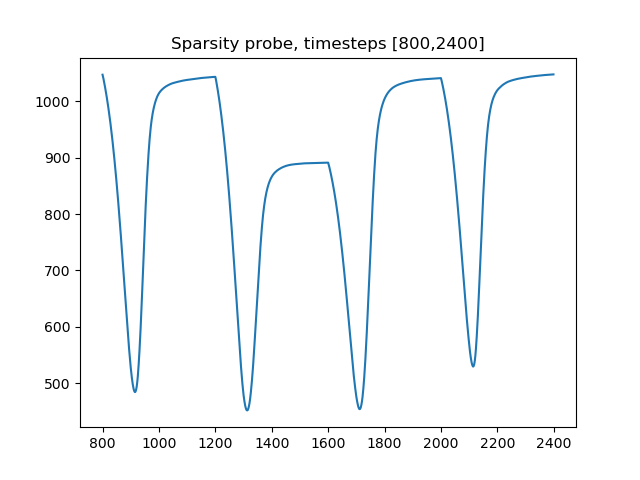

---

The evolution of the sparsity cost over four 400-timestep cycles.

---

At the beginning of a 400-timestep display period, the system is adapted to the previous image. As the system evolves for the new image, image patches that no longer explain the data are outcompeted and their activity reduces to zero. At the same time, different image patches that better explain the data have their internal state u begin to increase. However, the transfer function has a threshold λ, so that the new neurons do not activate immediately. This explains the decrease in the sparsity penalty at the beginning of the display period. Eventually, the newly excited neurons reach the threshold and begin to activate. As they do so, the sparsity penalty increases, although this increase is outweighed by the improvement in reconstruction. The system now settles down toward a new steady-state that encodes the new input. This slow convergence continues until the next display period, when the equilibrium is once again changed, and the cycle repeats.

In the preceding run, we processed several images, but serially. We next explore how to work in parallel.

2. Data Parallelism

We can make use of data parallelism by setting the nbatch parameter. This parameter controls how many images are sparse coded at once. Make a new .lua file from the Multiple_Images.lua file and edit it to change the nbatch parameter.

$ cp input/LCA_CIFAR_Multiple_Images.lua input/LCA_CIFAR_NBatch.lua

In the input/LCA_CIFAR_NBatch.lua file, change the line

local nbatch               = 1;   --Number of images to process in parallel 

to

local nbatch               = 16;  --Number of images to process in parallel 

The numImages value does not have to be a multiple of the nbatch value; however, images will be taken in batches of the given size, so that the number of images processed will be rounded up to the next value of nbatch.

Also change the output path from

local outputPath           = "output_multiple_images";

to

local outputPath           = "output_nbatch";

We once again generate the .params file and run OpenPV.

$ lua input/LCA_CIFAR_NBatch.lua > input/LCA_CIFAR_NBatch.params
$ ../tests/BasicSystemTest/Release/BasicSystemTest -p input/LCA_CIFAR_NBatch.params -l LCA-CIFAR-run.log -t 2

If you now list the contents of the ouput_nbatch directory, you should see that there now 16 probe files for each probe, indexed from 0 through 15. The run went for 400 timesteps, and processed 16 images instead of one during that time. We can use the batch_element argument of the readenergyprobe or readlayerprobe function to read multiple batch elements of the same probe at once.

$ python
>>> import pvtools
>>> energydata = pvtools.readenergyprobe(
...   'TotalEnergyProbe',
...   directory='output_nbatch',
...   batch_element=range(16))
>>> energydata['time'].shape
(400,)

>>> energydata['values'].shape
(400, 16)

The 'values' field of energydata contains the probe values for each of the 16 elements. It is also possible to pass a list to the batch_element argument, to read some but not all of the batch elements. Let's plot the energy probe values.

>>> import matplotlib.pyplot
>>> matplotlib.interactive(True)
>>> matplotlib.pyplot.figure()
>>> matplotlib.pyplot.plot(energydata['time'], energydata['values'])
>>> matplotlib.pyplot.title('Total Energy, 16 images, parallel')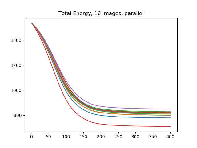

---

The energy cost function for the 16 images processed in parallel.

---

We describe the previous run as parallel because during each timestep of LCA, each of the 16 images were updated. This is in contrast to the earlier multiple_images run where the 16 images were handled sequentially: one image was processed during the first 400 timesteps, the second from timesteps 401 through 800, and so on. However, the computer is handling the batch sequentially within each timestep. We now turn to using MPI to spread the batch across several processes.

We will create a new .params file, as usual, but now the only change we need to make is to the outputPath parameter. The parallelism is defined on the command line when we call the PetaVision executable.

$ cp input/LCA_CIFAR_NBatch.lua input/LCA_CIFAR_Data_Parallelism.lua

In input/LCA_CIFAR_Data_Parallelism.lua file, change the line

local outputPath           = "output_nbatch";

to

local outputPath           = "output_data_parallelism";

and generate the .params file:

$ lua input/LCA_CIFAR_Data_Parallelism.lua > input/LCA_CIFAR_Data_Parallelism.params

We must now decide how many processes to spread the batch over; it must be a divisor of nbatch and it should also be no bigger than the number of cores available on your machine. We will use 8 in our example; for a smaller machine you might want to choose 4, or for a bigger machine you could choose 16.

We modify the command in two places. First, we use the mpiexec command to run under MPI, and specify the number of processes. An MPI implementation's mpiexec command might take either -n or -np to specify the number of processes; in the command below use whichever option is correct for your system. Second, we add -batchwidth 8 to the options passed to the PetaVision excecutable. Note that there is a single hyphen, not a double hyphen. The space between -batchwidth and the number of processes is required.

The reason we have to specify the number of processes both as a batchwidth argument and as an argument to mpiexec is that there are other ways we can use MPI, as we will see in the model parallelism section, below.

$ mpiexec -np 8 ../tests/BasicSystemTest/Release/BasicSystemTest -p input/LCA_CIFAR_Data_Parallelism.params -batchwidth 8 -l LCA-CIFAR-run.log -t 2

3. Model Parallelism

The CIFAR-10 images are 32x32x3, and in the PetaVision run, the sparse coding layer is 16x16x128. We can use MPI to divide the run into several rows and columns, as long as the division splits each layer into equally sized pieces. The features, however, cannot be split across MPI processes; each process handles all the features in its part of the layer.

For example, we can divide the run into two rows and four columns, because then each process takes a 4x8x128 section of the leaky integrator layer, and an 8x16x3 section of the other layers. However, we could not use three rows, because none of the layers' vertical dimension is a multiple of three.

As in the case of data parallelism, we do not need to modify the input parameters to use model parallelism. However, we will change the outputPath parameter as usual.

$ cp input/LCA_CIFAR_Data_Parallelism.lua input/LCA_CIFAR_Model_Parallelism.lua

In input/LCA_CIFAR_Data_Parallelism.lua file, change the line

local outputPath           = "output_data_parallelism";

to

local outputPath           = "output_model_parallelism";

and generate the .params file:

$ lua input/LCA_CIFAR_Model_Parallelism.lua > input/LCA_CIFAR_Model_Parallelism.params

To use MPI for model parallelism, we use the options -rows and -columns as arguments to the PetaVision executable.

Run-time flag	Description
-rows numRows	Split each layer into this many rows.
-columns numColumns	Split each layer into this many columns.

The number of MPI processes must equal numRows * numColumns. In the example below, we use two rows and two columns, for a total of four MPI processes.

$ mpiexec -np 4 ../tests/BasicSystemTest/Release/BasicSystemTest -p input/LCA_CIFAR_Model_Parallelism.params -columns 2 -rows 2 -l LCA-CIFAR-run.log -t 2

4. Using Both Data and Model Parallelism

It is possible to use both data and model parallelism in the same run, by setting the batchwidth, rows, and columns options simultaneously. The number of MPI processes must equal the product of the rows, columns, and batchwidth arguments. As usual, we create a new params file with a new outputPath value.

$ cp input/LCA_CIFAR_Model_Parallelism.lua input/LCA_CIFAR_Full_Parallelism.lua

In input/LCA_CIFAR_Full_Parallelism.lua file, change the line

local outputPath           = "output_model_parallelism";

to

local outputPath           = "output_full_parallelism";

and generate the .params file:

$ lua input/LCA_CIFAR_Full_Parallelism.lua > input/LCA_CIFAR_Full_Parallelism.params

Now we run with 2 rows, 2 columns, and batchwidth 2. This means that each process will work on eight of the sixteen images, and will work on one quarter (half vertically and half horizontally) of each image that it handles.

$ mpiexec -np 8 ../tests/BasicSystemTest/Release/BasicSystemTest -p input/LCA_CIFAR_Full_Parallelism.params -columns 2 -rows 2 -batchwidth 2 -l LCA-CIFAR-run.log -t 2

We note here that it is not necessary to specify all three of the options -rows, -columns, and -batchwidth. If only two are specified, the third is inferred from the number of processors. However, note that the run will fail if the number of processors is not a multiple of the product of the two options that were specified.

If either -rows or -columns is specified but the other is not, and -batchwidth is not specified, the batchwidth is taken to be 1, and the other option is chosen so that numRows * numColumns is the number of processes.

If -batchwidth is specified but neither -rows nor -columns is specified, the program tries to choose -rows and -columns so that they are close to sqrt(numProcesses/batchWidth) and their product is numProcesses/batchWidth. It may not come up with a suitable choice of options, even if a suitable choice exists.

Finally, if none of -rows, -columns, or -batchwidth is present, the program proceeds adds the option -batchwidth 1 and attempts to choose -rows and -columns as described above.

5 Conclusion

In this page, we saw how to use PetaVision to sparse code several images in parallel. Up to this point, we have been using random initial weights that are specified start of the run and remain fixed. In the next part of the tutorial (currently under development), we will see how to have PetaVision update the weights to improve the sparse coding.